“Online” data assimilation (DA) is used to generate a seasonal-resolution reanalysis dataset over the last millennium by combining forecasts from an ocean–atmosphere–sea ice coupled linear inverse model with climate proxy records. Instrumental verification reveals that this reconstruction achieves the highest correlation skill while using fewer proxies in surface temperature reconstructions compared to other paleo-DA products, particularly during boreal winter when proxy data are scarce. Reconstructed ocean and sea ice variables also have high correlation with instrumental and satellite datasets. Verification against independent proxy records shows that reconstruction skill is robust throughout the last millennium. Analysis of the results reveals that the method effectively captures the seasonal evolution and amplitude of El Niño events, seasonal temperature trends that are consistent with orbital forcing over the last millennium, and polar-amplified cooling in the transition from the medieval climate anomaly to the little ice age.
Many paleoclimate records are sensitive to a particular season. Annual averaging can obscure that information. LMR Seasonal preserves four seasons per year and uses a coupled forecast model to carry information from one season into the next.
The result is a gridded paleoclimate reanalysis of surface air temperature, sea surface temperature, upper-ocean heat content, and Northern Hemisphere sea ice. It supports research on ENSO evolution, seasonal temperature trends, and multicentennial climate change.
Three results, with the figures and context behind them.
01
Seasonal information improves winter reconstruction.
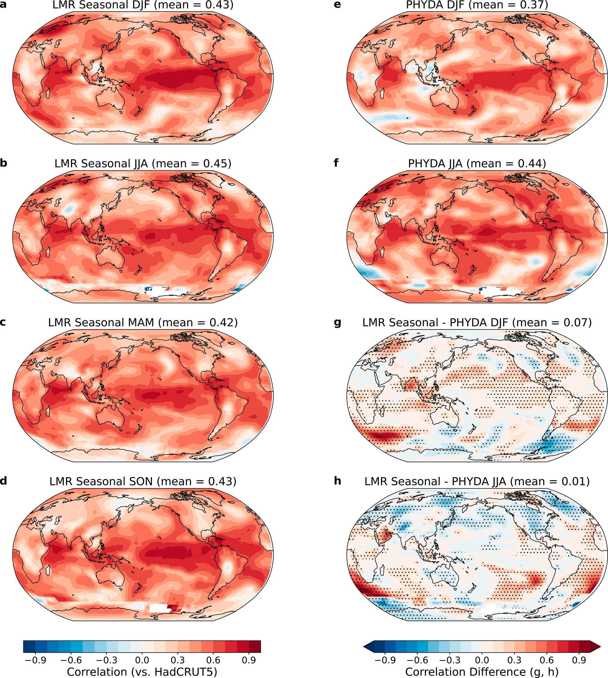
Against HadCRUT5 over 1880–2000, LMR Seasonal reconstructs surface temperature in all four seasons. Compared with PHYDA, its relative advantage is more pronounced in boreal winter, when temperature-sensitive proxies are sparse.
The comparison varies by region and season: PHYDA performs better in parts of North America and Eurasia during summer. The figure maps those differences rather than implying a uniform improvement.
Fig. 4 · Seasonal temperature verification. Left: LMR Seasonal in all four seasons. Right: PHYDA and correlation differences for DJF and JJA. Black dots in the difference maps indicate significance at the 95% level. Verification period: 1880–2000.
02
El Niño emerges as an evolving event.
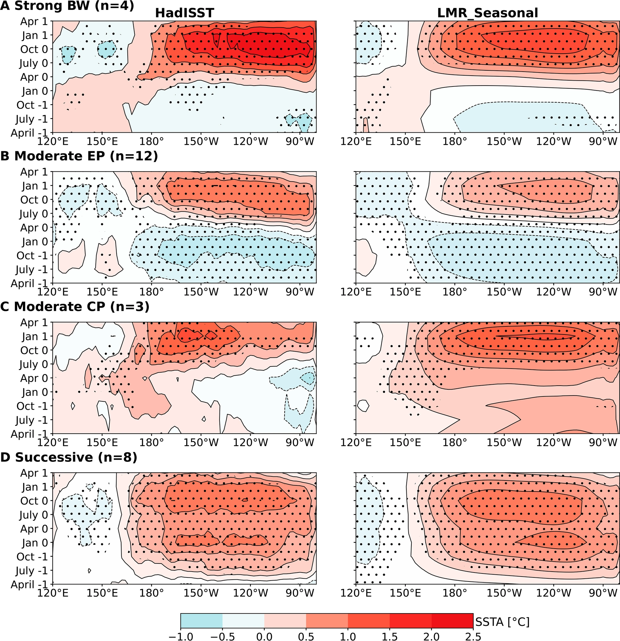
The reconstruction captures much of the seasonal evolution of four El Niño onset classes in the instrumental period, including strong basin-wide, moderate eastern-Pacific, moderate central-Pacific, and successive events.
Reconstructed amplitudes are smaller for some classes. The central-Pacific comparison is based on only three events during 1900–2000. These modern comparisons help assess the reconstruction before using the longer record to study ENSO.
Fig. 10 · El Niño onset and evolution. HadISST (left) and LMR Seasonal (right), using events from 1900–2000. Rows show the four event classes; dots indicate composite anomalies significant at the 95% level. The color scale is SST anomaly in °C.
03
Long-term cooling has a seasonal and polar signature.
For 850–1850 CE, reconstructed cooling is greater in DJF and SON than in MAM and JJA, consistent with a delayed climate response to orbital-insolation trends. These trends emerge from proxy assimilation; trends were removed from the model training data.
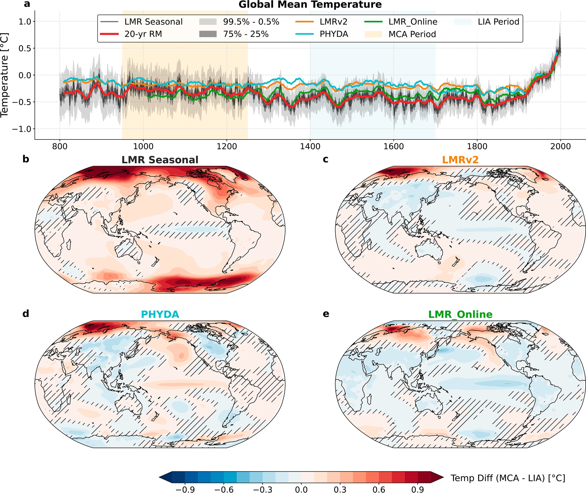
The reconstruction also resolves amplified high-latitude cooling from the Medieval Climate Anomaly (950–1250 CE) to the Little Ice Age (1400–1700 CE), alongside changes in Northern Hemisphere sea ice and upper-ocean heat content.
Fig. 14 · Medieval climate and the Little Ice Age. Top: global mean temperature, including 20-year running means and LMR Seasonal ensemble intervals. Maps: MCA minus LIA temperature. Hatching marks regions that do not pass the 95% significance test.
How the system works
Forecast. Update. Carry the memory forward.
01 / FORECAST
A coupled climate prior
A linear inverse model (LIM), trained on climate-model output, forecasts surface temperature, upper-ocean heat content, and Northern Hemisphere sea ice from one season to the next.
02 / ASSIMILATE
Proxies in their own seasons
Proxy system models connect tree rings, corals, and ice cores to climate variables. An ensemble Kalman filter updates the appropriate season or set of seasons using each record’s temperature sensitivity.
03 / CYCLE
Information persists
The updated climate state initializes the next forecast. Ocean and sea ice persistence help transmit proxy information into seasons with fewer records. Annual-mean proxies update the available seasonal states.
DJFDec–Feb→MAMMar–May→JJAJun–Aug→SONSep–Nov→ next year
Method: paper §2, Fig. 2 and Table 1. Instrumental verification uses temperature, ocean, and sea ice reference datasets. Independent-proxy verification withholds 20% of proxies across 50 bootstrap experiments (§3b, Fig. 12).
Use the reconstruction
Open data. A practical starting point.
NetCDF files · 800 ensemble members Four seasonal means per year
The published files cover 800–2000 CE. Global temperature and ocean fields use a 90 × 180 grid; Northern Hemisphere sea ice fields use a 45 × 180 grid. Both have 2° spacing.
Start with one climate-index file. The example calculates the ensemble mean and interquartile range for 1900–2000.
Use cftime to decode the full record, including early dates. File timestamps in January, April, July, and October label DJF, MAM, JJA, and SON, respectively; these are three-month averages. DJF includes December of the previous year.
from pathlib import Path
from urllib.request import urlretrieve
import xarray as xr

path = Path("Nino34_ens.nc")
if not path.exists():
    urlretrieve(
        "https://atmos.uw.edu/~zilumeng/LMR_Seasonal/"
        "data/index/Nino34_ens.nc", path
    )

with xr.open_dataset(path, use_cftime=True) as ds:
    nino = ds["Nino34"].sel(time=slice("1900", "2000"))
    mean = nino.mean("ens_num")
    iqr = nino.quantile([0.25, 0.75], dim="ens_num")
    print(mean)
    print(iqr)
Data license: CC BY 4.0. Code license: BSD 3-Clause. For a first look, use the ensemble means or indices; the full gridded ensemble is approximately 2 TB.
Selected research uses
How other studies use this work
Independent studies that cite Meng, Hakim & Steig (2025), with the specific use documented in each paper.
Sjolte & Tao (2026) · Climate of the Past, 22, 915–933
Compares LMR Seasonal summer and winter temperatures with a North Atlantic reconstruction spanning 1241–1970, examining spatial agreement and how it changes through time.
Compares LMR Seasonal with a new Yangtze River Basin summer temperature dataset and observations to evaluate regional temperature patterns and variability.
Chen et al. (2026) · Nature Communications, 17, 3234
Uses LMR Seasonal alongside other reconstructions to assess simulated temperature variability and long-term trends in China for a millennial land-carbon study.
Lin et al. (2026) · Journal of Advances in Modeling Earth Systems, 18(7), e2026MS005767
Cites Meng et al. (2025) for two choices in its linear inverse model: retaining 15 principal components per variable and handling negative noise-covariance eigenvalues while preserving total variance.
Selected examples, checked 4 October 2026; this is not a complete citation list. Data comparisons and methodological citations are identified separately. For references to include in your own work, see Cite this work.
Scope & interpretation
Read the skill alongside the result.
Based on paper §§2–5.
Seasonal climate fields. Four three-month averages per year support seasonal-to-multicentennial analyses. This dataset does not resolve daily weather or individual storms.
Regional skill varies. Sparse proxies and model teleconnections limit some regions, including the Southern Ocean. Modern verification does not provide equally direct constraints for every earlier year.
Northern Hemisphere sea ice. Southern Hemisphere sea ice is not reconstructed. Sea ice skill varies by location and season; the framework was not specifically optimized for sea ice.
Ensemble means smooth variability. Averaging can reduce event amplitudes and temporal variance. Retain ensemble information when drawing conclusions about individual events or uncertainty.
Coupled statistical dynamics. The LIM describes climate anomalies using relationships learned from model output. Interpret patterns together with proxy coverage, validation, and the assumptions of the reconstruction.
Use Meng, Hakim & Steig (2025) when discussing the seasonal reconstruction, method, or scientific results. Cite the final Journal of Climate article for the published findings.
ANALYZING THE DATA
Cite the paper and data source
Also cite the dataset DOI and version when using the archived ensemble means. For indices or full members from the UW portal, record the portal URL, files used, and download date.
USING THE CODE
Cite the paper and code version
The repository requests a citation to the paper. Also identify the code repository and the commit or release used, so readers can locate your implementation.
Published paper
Meng, Z., G. J. Hakim, and E. J. Steig, 2025: Coupled Seasonal Data Assimilation of Sea Ice, Ocean, and Atmospheric Dynamics over the Last Millennium. Journal of Climate, 38(23), 7229–7247. doi:10.1175/JCLI-D-25-0048.1.
Archived ensemble-mean data: Meng, Z., G. J. Hakim, and E. J. Steig, 2025: Last Millennium Reanalysis (LMR) Seasonal: A Millennium of Climate Data, version v1. Zenodo. doi:10.5281/zenodo.17268597. Indices and full ensemble members are available separately through the UW portal.
BibTeX · published article
@article{Meng2025LMRSeasonal,
  author  = {Meng, Zilu and Hakim, Gregory J. and Steig, Eric J.},
  title   = {Coupled Seasonal Data Assimilation of Sea Ice, Ocean,
             and Atmospheric Dynamics over the Last Millennium},
  journal = {Journal of Climate},
  year    = {2025},
  volume  = {38},
  number  = {23},
  pages   = {7229--7247},
  doi     = {10.1175/JCLI-D-25-0048.1}
}
BibTeX · archived ensemble-mean dataset
@misc{Meng2025LMRSeasonalData,
  author    = {Meng, Zilu and Hakim, Gregory J. and Steig, Eric J.},
  title     = {Last Millennium Reanalysis (LMR) Seasonal:
               A Millennium of Climate Data},
  year      = {2025},
  publisher = {Zenodo},
  note      = {Version v1; ensemble-mean archive},
  doi       = {10.5281/zenodo.17268597},
  url       = {https://doi.org/10.5281/zenodo.17268597}
}
The arXiv link is the January 2025 preprint. For the final results and citation, use the published Journal of Climate article linked above. Figures on this page are from the published paper.