Empirical Orthogonal Function

Parameter

• data (np.ndarray): shape (time, * space grid number)

• weights : shape (* space grid number , or can be broadcast to space grid number)

Method

• solve: solve the EOF results of data

  args:

  method (str): ‘svd’ or ‘eig’ or ‘dask_svd’

  if ‘dask_svd’, use dask to solve , another parameters are also required. dim_min: the minimum patterns of data to be solved

  chunks: the chunks to split data in the dask

  if ‘svd’, use numpy to solve

  if ‘eig’, use numpy to solve
• north_test: north test of EOF results

  args:

  npt (int): number of modes to be tested

  perc (Bool): if True, return the proportion of error

  return:

  typical errors of each pattern

• get_pc(npt): get princple components of first npt modes

• get_pt(npt): get spatial patterns of first npt modes

• get_eign: get eign values of EOF result

• get_varperc: get the proportion of mode variance

• load_pt: load space patterns of extral data rather than from solving

• decoder: project pcs on patterns to get original fields

Example

load Modules

import sacpy as scp
import numpy as np
import matplotlib.pyplot as plt

Get SST and SSTA data

sst = scp.load_sst()["sst"].loc[:, -20:30, 150:275]
ssta = scp.get_anom(sst)

EOF Calcualtion

eof = scp.EOF(ssta)
eof.solve(method='dask_svd', chunks={'time': 1000}, dim_min=10)
# or
eof.solve()
# or
eof.solve(method='svd')
# or
eof.solve(method='eig')

Get EOF result

# get pc and pattern
pc = eof.get_pc(npt=2)
pt = eof.get_pt(npt=2)
# get proprtion of mode variance
eof.get_varperc(npt=3)

array([0.53846117, 0.1339264 , 0.06592592])

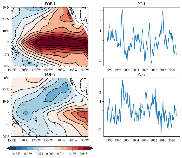
Plot the EOF Results

import cartopy.crs as ccrs
import sacpy.Map
lon , lat = ssta.lon , ssta.lat
# =========================set figure================================
fig = plt.figure(figsize=[9,7])
# =========================     ax  ================================
ax = fig.add_subplot(221,projection=ccrs.PlateCarree(central_longitude=180))
m1 = ax.scontourf(lon,lat,pt[0,:,:],cmap='RdBu_r',levels=np.linspace(-0.75,0.75,15),extend="both")
ax.scontour(m1,colors="black")
ax.init_map(smally=2.5)
ax.set_title("EOF-1")
# =========================    ax2  ================================
ax2 = fig.add_subplot(222)
ax2.plot(sst.time,pc[0])
ax2.set_title("PC-1")
# =========================    ax3  ================================
ax3 = fig.add_subplot(223,projection=ccrs.PlateCarree(central_longitude=180))
m2 = ax3.scontourf(lon,lat,pt[1,:,:],cmap='RdBu_r',levels=np.linspace(-0.75,0.75,15),extend="both")
ax3.scontour(m2,colors="black")
ax3.init_map(smally=2.5)
ax3.set_title("EOF-2")
# =========================   ax4   ================================
ax4 = fig.add_subplot(224)
ax4.plot(sst.time,pc[1])
ax4.set_title("PC-2")
# =========================  colorbar  ================================
cb_ax = fig.add_axes([0.1,0.03,0.4,0.02])
fig.colorbar(m1,cax=cb_ax,orientation="horizontal")

<matplotlib.colorbar.Colorbar at 0x15e776f20>

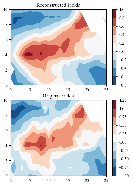
Reconstruction use PT and patterns

eof = scp.EOF(ssta)
eof.solve()
pc = eof.get_pc(npt=10)
pt = eof.get_pt(npt=10)
# eof.load_pt(pt)
res = eof.decoder(pc.T)
plt.figure(figsize=[5,7])
plt.subplot(211)
plt.title("Reconstructed Fields")
plt.contourf(res[0])
plt.colorbar()
plt.subplot(212)
plt.title("Original Fields")
plt.contourf(ssta[0])
plt.colorbar()

<matplotlib.colorbar.Colorbar at 0x15edce5c0>